Introduction to R for Business Analytics

Classification via Mathematical Functions

In the following pages we will see different ways how we can use mathematical functions to achive classification.

Review: Classificaton Trees

A quick review of classificaton trees:

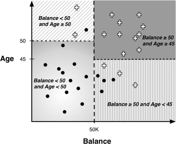
Decision barriers are perpendicular to the axis. Is there another way we can classify this data?

Linear Discrimination

By being able to draw a line that is still straight, but not perpendicular, we can better divide the space:

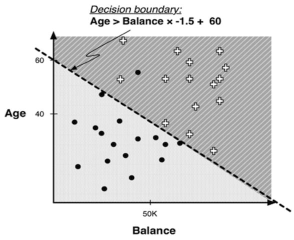
The new decision boundary is essentially a weighted sum of the values of the various attributes:

Basic Linear Model Structure

Most function fitting techniques are based on this one model. It is taking multiple attributes into account through one mathematical formula – know as a parameterized model.The general formula is: \(f(x) = w_0 + w_1x_1 + w_2x_2 + ...\) Where w0 is the intercept, wi are the weights (parameters) and xi are the individual component features.

Depending on the value of the weights/parameters, however, the results (below) can be quite different:

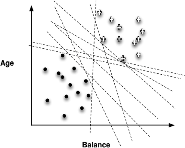
The task of the data mining procedure is to “fit” the model to the data by finding the best set of parameters, in some sense of “best.”

Objective Function

How can we chose a suitable objective function?

First step: Determine the goal or objective of choosing parameters – this helps determine the best objective function.

Objective Function examples:

• Linear regression, logistic regression, and linear discriminations such as support-vector machines

Then, find optimal value of the weights by maximizing and minimizing the objective function.

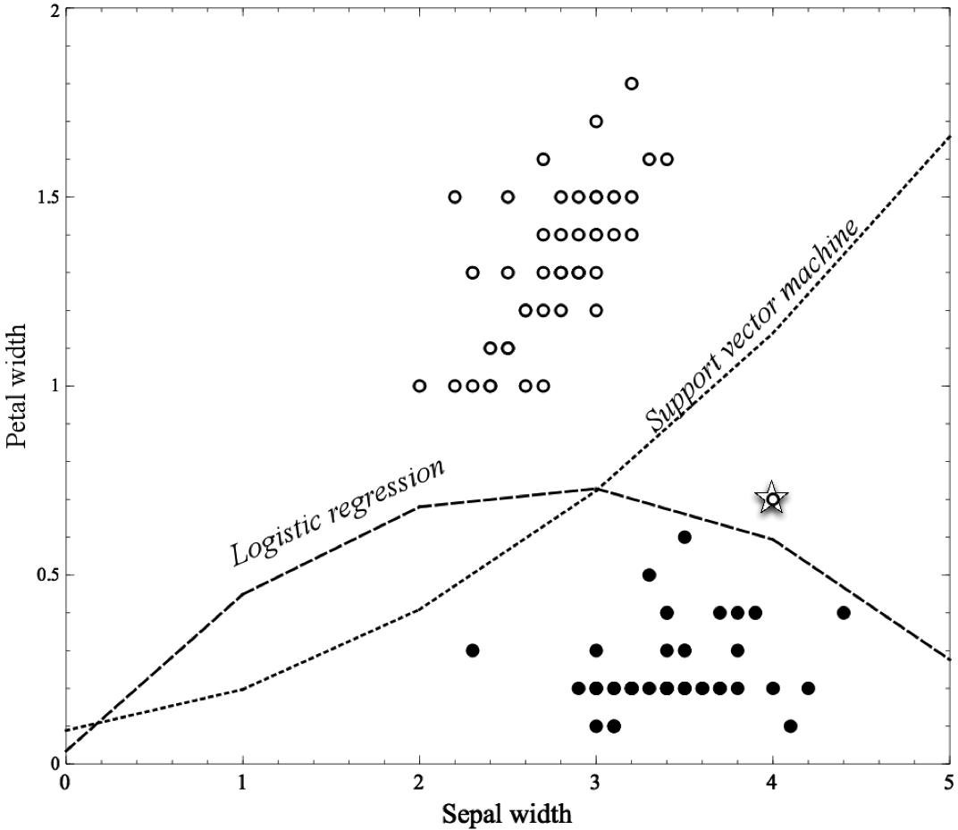
Iris Example

Below is a classification example using the Iris Dataset (available as data(iris) in R).

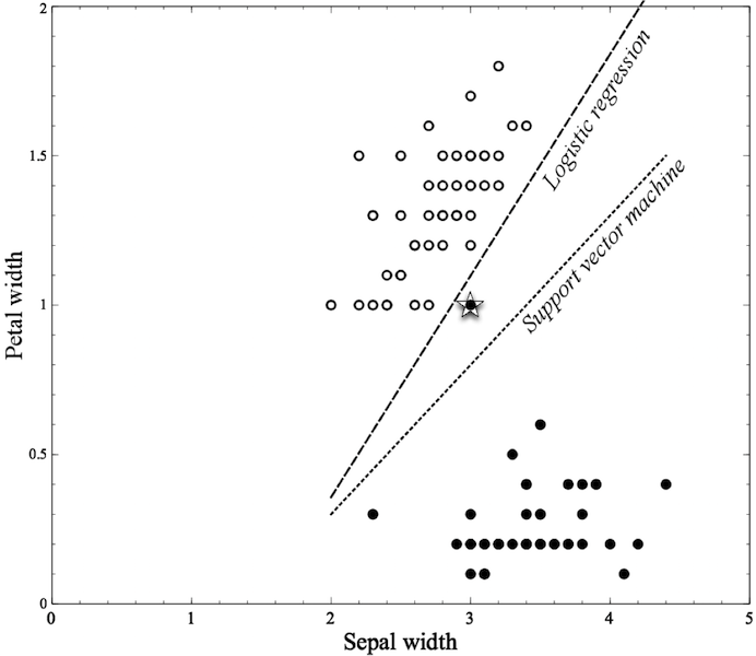
Mining a linear discriminant from data. Two different objectives are shown. Note how they divide and classify data differently.

Support Vector Machines

Goal is to maximize the margin or the space between the two dashed lines. The linear discriminant (solid line below) is the center between the two dashed lines.

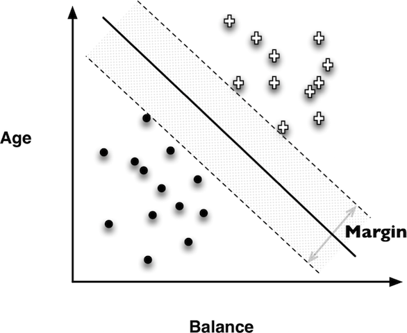
If data cannot be linearly separated, the best fit is a balance between a fat margin and a low total error penalty.

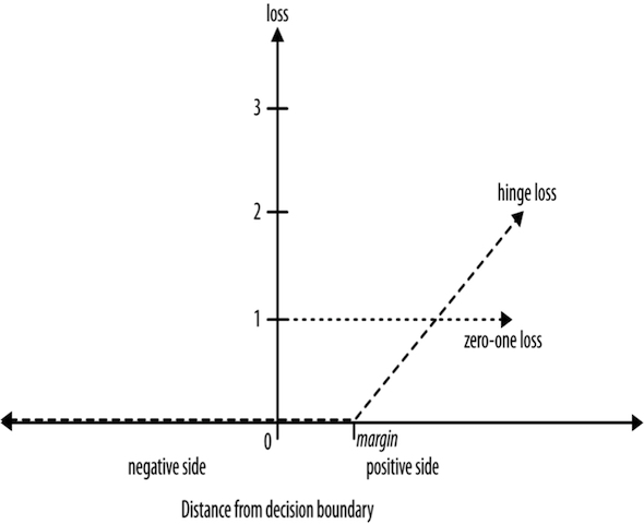
Loss Functions

Hinge Loss: incurs no penalty for an example that is not on the wrong side of the margin. The hinge loss only becomes positive when an example is on the wrong side of the boundary and beyond the margin. Loss then increases linearly with the example’s distance from the margin, thereby penalizing points more the farther they are from the separating boundary.

Zero-one loss: assigns a loss of zero for a correct decision and one for an incorrect decision.

Regression via Mathematical Functions

Objective Functions for Linear Models:

Absolute Error method:

• Minimize the sum of the absolute errors to find the optimal function

Squared Error method:

• Minimize the sum of the squares of these errors
• Convenient mathematically
• Strongly penalizes very large errors

Both have pros/cons - depends on the business application.

Class Probability Estimation and Logistic Regression

Logistic regression is an objective function used to estimate probability of something occurring (Ex. Probability of bank fraud).

In order to fit a linear model the distance from the decision boundary needs to be between \(-\infty\) and \(\infty\), but probabilities only go between zero and one.

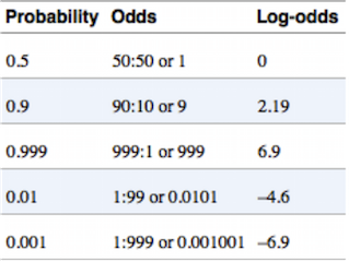
The problem can be solved by taking the logarithm of the odds (log-odds) because for any number zero to \(\infty\), its log odd will be between \(-\infty\) and \(\infty\).

See below:

Log Odds Linear Function:

\(log (\frac{p+(x)}{1-p+(x)}) = f(x) = w_0 + w_1x_1 + w_2x_2 + \ldots\)

Where \(p + (x)\) is the estimate of a particular event occuring.

The Logistic Function:

\(p+(x) = \frac{1}{1+e^{-f(x)}}\)

Graph of a Logistic Function:

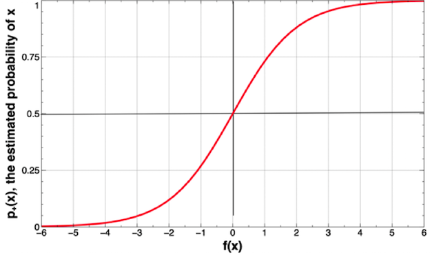
Note: The further away from the decision boundary \((x=0)\), the more certain the model

Logistic regression vs. Tree Induction

• Models will likely have different levels of accuracy

• It is difficult to determine which method is more effective at the beginning of the experiment

• Data science team doesn’t always have ultimate say in which model is used - stakeholders must agree

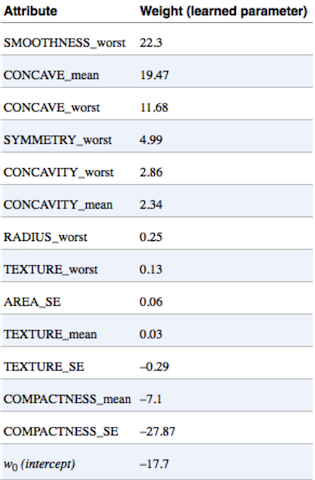
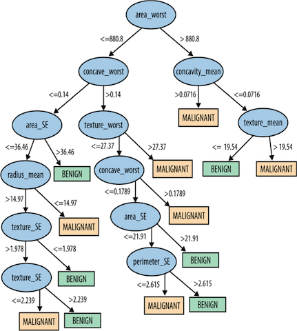
Example: Wisconsin Breast Cancer Dataset

Learned by Logistic Regression:

---

Classification Tree:

---

Results:

Linear equation learned by logistic regression

• 98.9% accuracy

• Only 6 mistakes total

Classification tree model

• 99.1% accuracy

• One mistake out of 569 samples

Which is better?

• Model evaluation will be discussed in the following chapters, but what is important now is to recognize that they produce different results

Nonlinear Functions, Support-Vector Machines, and Neural Networks

Nonlinear Functions: The two most common families of techniques that are based on fitting the parameters of complex, nonlinear functions are nonlinear support-vector machines and neural networks.

Nonlinear support vector machines are essentially a systematic way of adding more complex terms (ex. Sepal width\(^2\)) and fitting a linear function to them.

Neural networks can be thought of as a “stack” of models. We could think of this very roughly as first creating a set of “experts” in different facets of the problem (the first-layer models), and then learning how to weight the opinions of these different experts (the second-layer model).

UCI Iris Example, revisited with \(Sepal width^2\)

The Iris dataset with a nonlinear feature. In this figure, logistic regression and support vector machine—both linear models—are provided an additional feature, Sepal width\(^2\), which allows both the freedom to create more complex, nonlinear models (boundaries), as shown.

Note on Nonlinear Functions:

Be careful! As we increase the flexibility of being able to fit the data, we increase the risk of the data fitting too well. The concern is that the model will fit well to the training data, but not be general enough to apply to data drawn from the same population or application

Summary

In this chapter we:

• Introduced a 2nd predictive modeling technique called function fitting or parametric modeling
• Learned how to determine and optimize function parameters and define the objective function
• Investigated linear modeling techniques including: traditional linear regression, logistic regression, and linear discriminants such as support-vector machines
• Compared tree induction with function fitting
• Investigated nonlinear functions including nonlinear support-vector machines and neural networks
• Introduced the concept of “overfitting”