Introduction to Predictive Modeling

Introduction to Predictive Modeling
Overview
Fundamental concepts covered in this module
- Identifying informative attributes
- Segmenting data by progressive attribute selection
Exemplary techniques:
- Finding correlations
- Attribute/variable selection
- Tree induction
Objectives
After completing this module, students should be able to:
- Describe the basic underlying idea behind predictive modeling
- Compute entropy and information gain for a given dataset
- Read decision trees and decision rules
- Interpret decision trees and decision rules
- Perform inductive tree learning
- Evaluate the quality of a model such as a decision tree or regression
Business Understanding
Building on churn example: let’s think of predictive modeling as supervised segmentation.
Question we want to ask: How can we segment the population into groups that differ from each other with respect to some quantity of interest?
Target could be something we like to avoid (e.g., churn, write-offs, turbine failure) or something we would like to see (e.g., respond to offer).
Supervised Data Mining
Key (part 1): is there a specific, quantifiable target that we are interested in or trying to predict?
Examples:
- What will the IBM stock price be tomorrow? (e.g., $200)
- What would you do if you could predict this?
- Will this prospect default her loan? (e.g. yes/no)
- What would you do if you could predict this?
- Do my customers naturally fall into different groups
- Unsupervised: no objective target stated.
- What would you do if you could predict this?
Key (part 2): do we have data on this target?
Supervised data mining requires both parts 1 & 2
We don’t need the exact data (e.g., whether the current customers will leave) BUT we need data for the same or a related phenomenon (e.g., from customers from last quarter)
We will then use these data to build a model to predict the phenomenon of interest.
Question to ask: Is the phenomenon of “who left the company” last quarter the same as the phenomenon of “who will leave the company” next quarter?
Question to ask: Who might buy this completely new product I have never sold before?
Key (part 3): the result of supervised data mining is a MODEL that given data predicts some quantity
Model could be some rule:
  if (income <50K)
     then no Life Insurance
else Life Insurance- You can then apply this model (i.e., the rule) to any customer and it provides you a prediction
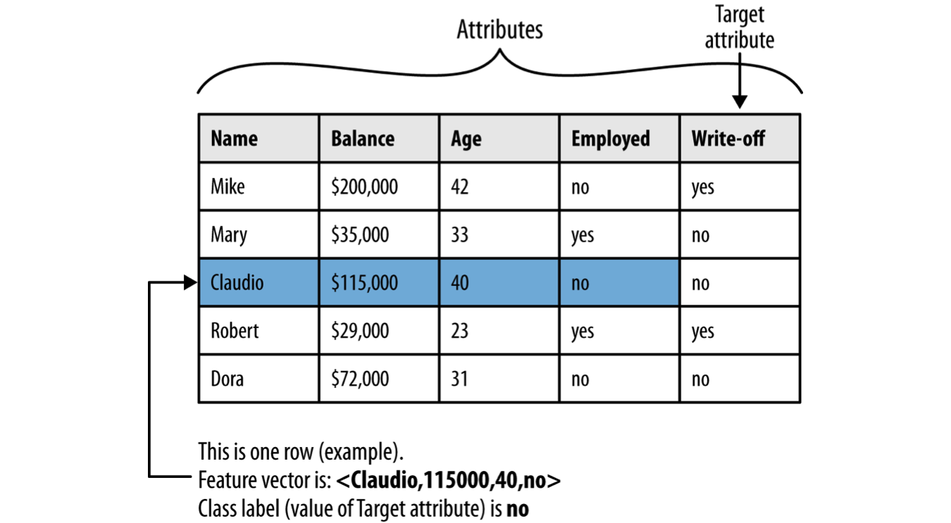
Terminology for supervised classification problem. The problem is supervised because it has target attribute and some training data. Classification because target is a category (yes/no) rather than numeric.
Within supervised learning: classification vs. regression
The difference is the type of target available:
Classification \(\Rightarrow\) categorical target (in historical data)
Regression \(\Rightarrow\) numerical target
Supervised Segmentation
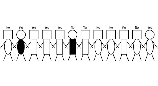
- Target: The yes/no associated with each person.
- Predictors: Attributes of the person such as shape of head and body.
Intuition: How can we segment the population into subgroups that have different values of target variable? (and the same value within a group)?
Problem: How can we judge whether a variable contains important information about the target variable? How much?
Selecting Information Attributes
Which attributes are best suited to segment the data according to the target values? In the above example, would “round body” be a good predictor of the target attribute? Why or why not? Is it sufficient?
What does the data look like?
Target: Two classes (yes & no)
Predictor attributes: head (round, square); body-type (rectangular, oval); body-color (white, grey)
Which of the attributes would be best to segment these people into groups?
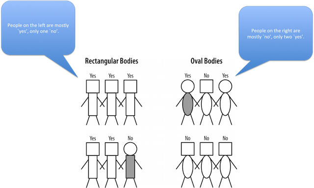
Challenges in Attribute Selection
- Attributes rarely split the group perfectly.
- Consider splitting by oval body to indicate “yes”
- Body color=grey would create pure segment (write-off=no ) if second person were not there
- Sometimes splits result in very small subsets (or even single observations)
- Does it make sense to make a segment for every numeric value? (No!) How can we create supervised segmentations using numeric attributes?
- Not all attributes are binary. E.g., numerical values could have many splits. How do we compare across variables that produce different number of splits?
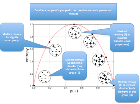
Splitting Criteria based on Information Gain called Entropy
- Entropy is measure of disorder
- Disorder corresponds to how mixed (impure) a segment is
- Group with many write-offs and many non-write-offs: has high entropy
- Very pure groups: low entropy
\(entropy = -p_1 log_2(p_1) - p_2 log_2(p_2) - \ldots - p_n log_2(p_n)\)
Selecting Information Attributes
Information Gain
Information gain: how much an attribute improves (or decreases) entropy over the whole segmentation it creates. i.e., information gain is change in entropy
\(IG(parent,children) = entropy(parent)-[p(c_1)entropy(c_1)+...]\)
Example #1
Write-off Example
Consider set \(S\) of 10 people with 7 of non-write-off class and 3 of write-off class:
\(p(non-write-off) = 7/10 = 0.7\)
\(p(write-off) = 3/10 = 0.3\)
\(entropy(S) = -[0.7*log_2(0.7)+.03 * log_2(0.3)]\)
\(entropy(S) = 0.88\)
This is the amount of information contained in the overall data.
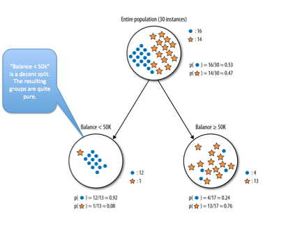
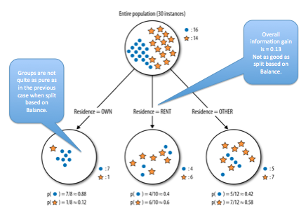
What is the information gain (IG) for splitting the data based on “balance 50k”?
How about splitting the data into three classes based on the Residence attribute?
Example #2
Example: Attribute Selection with Information Gain
Dataset: Mushroom Target: edible vs. poisonous
21 predictor variables
Which variable predicts the target? How well?
Intuition: Compute information gain from splitting the data based on different predictors.
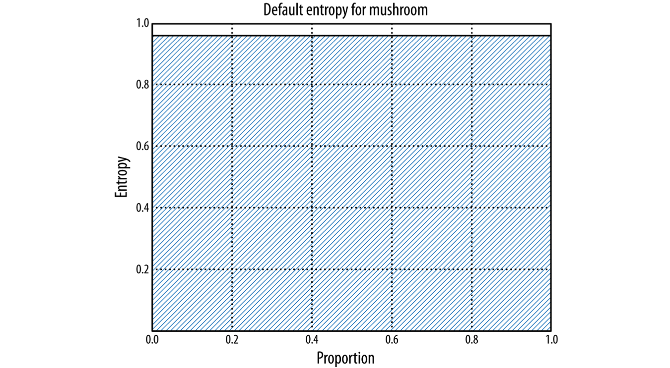
For Entropy charts below:
- X-axis: Proportion of the data that has a given value
- Y-axis: Entropy
- Shaded area: amount of entropy in the dataset when divided by some chosen attribute
- Goal: lowest entropy possible => as little shaded area as possible
Entropy chart of the entire dataset (no split):
Split by “Gill-Color”
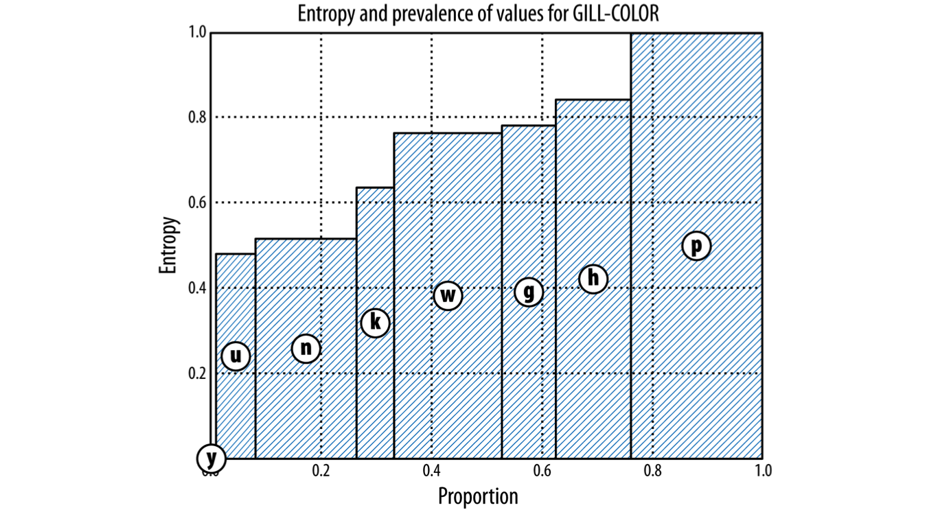
gill-color: black=k, brown=n, buff=b, chocolate=h, gray=g, green=r, orange=o, pink=p, purple=u, red=e, white=w, yellow=y
Split by Spore-Print-Color
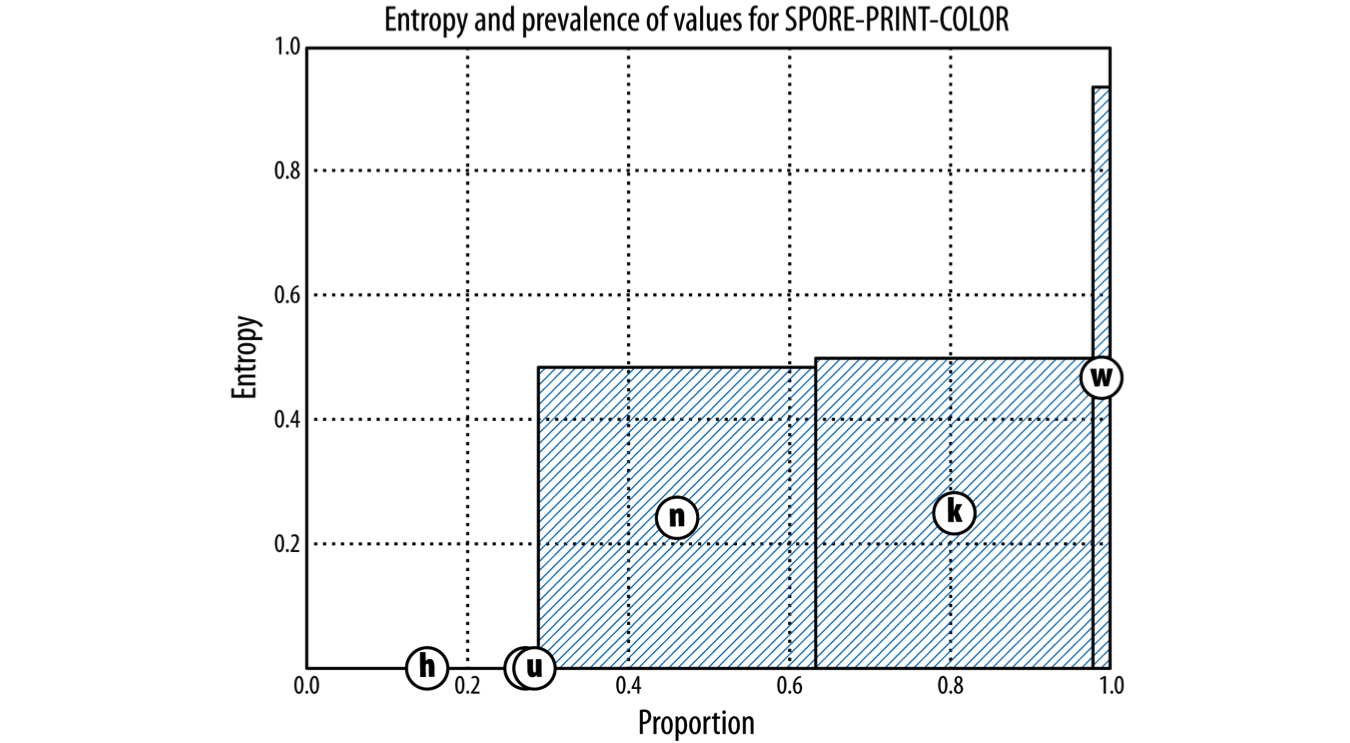
spore-print-color: black=k, brown=n, buff=b, chocolate=h, green=r, orange=o, purple=u, white=w, yellow=y
Split by Odor
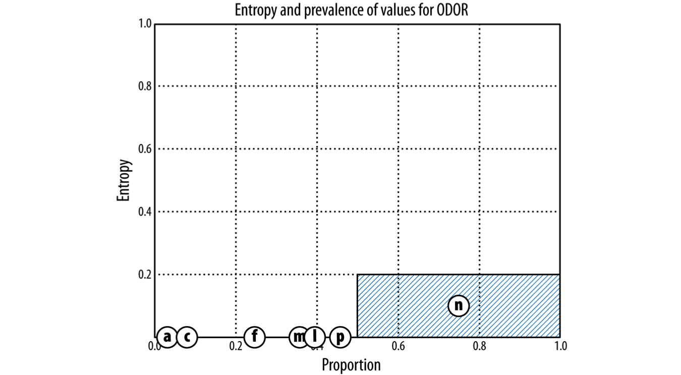
odor: almond=a, anise=l, creosote=c, fishy=y, foul=f, musty=m, none=n, pungent=p, spicy=s
Supervised Segmentation with Tree-Structured Models
‘Upside down tree’:
- root on top
- Nodes: interior nodes and terminal nodes (aka leafs)
- Each leaf corresponds to a segment of the data (i.e., value of the target attribute), and attributes and values along path give characteristics of segment
- This is called classification tree or decision tree
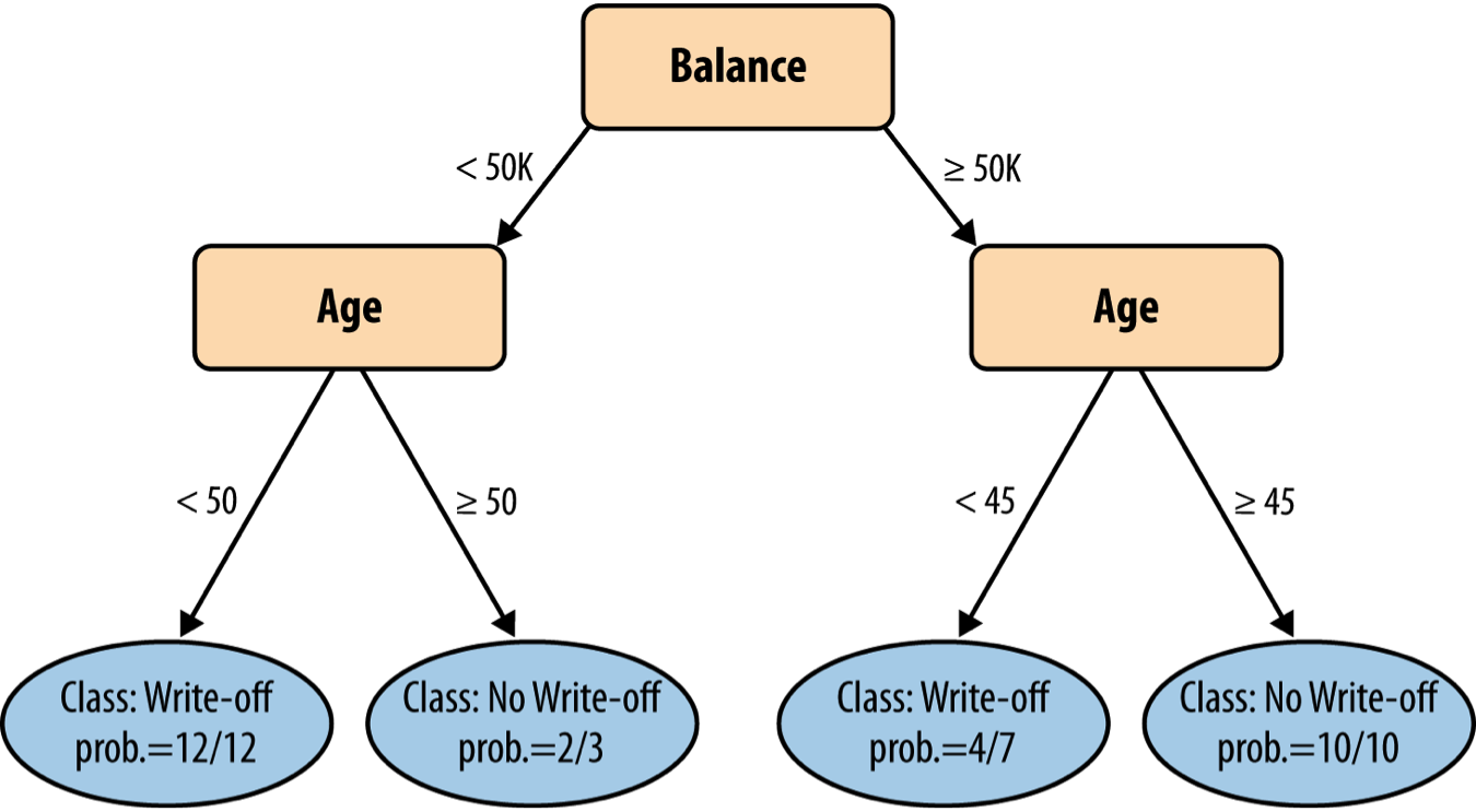
Simple decision tree for credit example
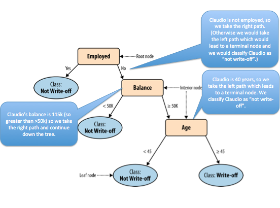
Exercise: Given the above decision tree, how would we classify the observation `Claudio’: Balance=115k, Employed=No, Age=40?
- Not Write-off
- We start at the root which asks “Is Claudio employed?” Since Claudio is not employed, we follow the right branch. The next nodes asks “What is Claudio’s current balance?”. The balance is given as $115K so this matches the \(\geq 50K\) condition so we again follow the right branch. Finally, the next node asks “How old is Claudio?” This is given as 40 years, which matches the \(< 45\) condition, so we follow the left branch. The left branch leads to a leaf node which gives the classification of the observation “Claudio” as Not Write-off.
- Write-off
- This is not correct. To classify the observation “Claudio” using the given decision tree, start at the root and follow each decision so that it matches the data given about Claudio. Can you try again?
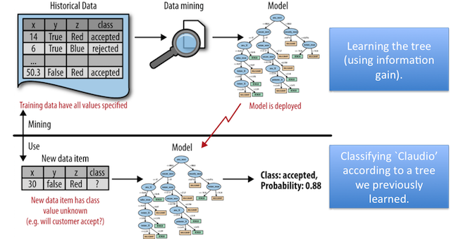
Recap: Difference between data mining and using data mining results
Tree Induction Example
Intuition: Starting with the whole dataset, continue to split the data based on different attributes to create the purest leaves possible (using the idea of information gain from above).
Ex: First Partitioning
First partitioning: splitting on body shape
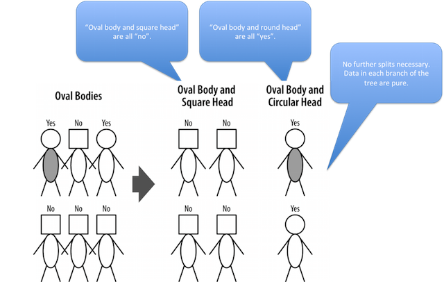
Ex: Second Partitioning
Second partitioning: the oval body people sub-grouped by head type
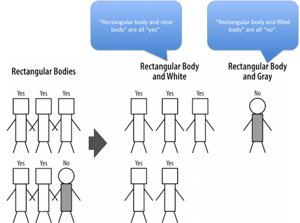
Ex: Third Partitioning
Third partitioning: rectangular body people subgrouped by body color
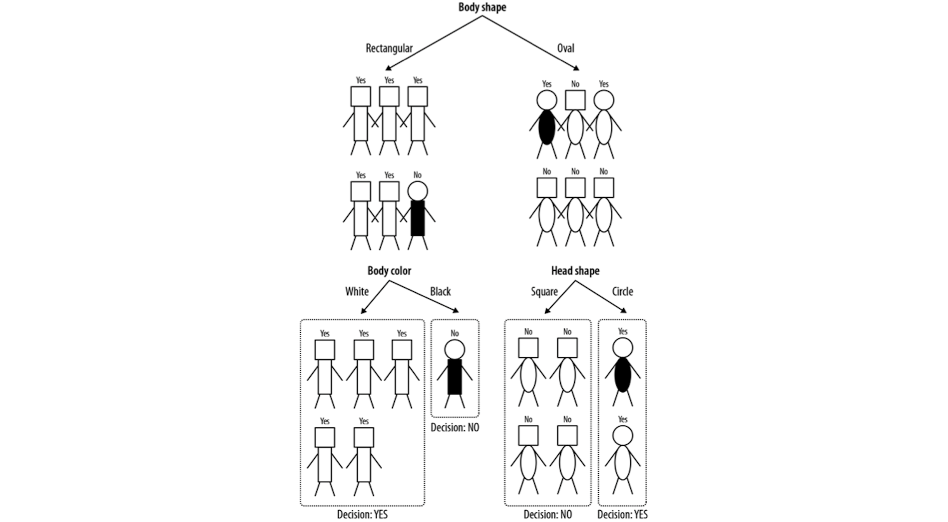
Ex: Complete Tree
The complete tree
Probability Estimation
Back to credit example: Probability estimation
Instead of simply classifying something as yes/no, write-off/non-write-off, we can also produce probability estimates: simply divide the number of the majority instances by the total number of instances in the segment. (This is called frequency-based class membership probability.)
One problem that arises is with segment with very small numbers of instances. If a leaf happens to have only a single instance, should we be willing to say that there is a 100% probability of that member of that segment will have the class that this one instance happens to have?
This phenomenon is one example of a fundamental issue in data science called “overfitting”: our predictions are very good but they are also tailored very closely to the specific dataset we were learning from. We will cover overfitting in more detail in a separate module.
One simple way to address it is the Laplace correction (see book p. 71 for details).
We can also visualize data observations according to the decision rules of our tree.
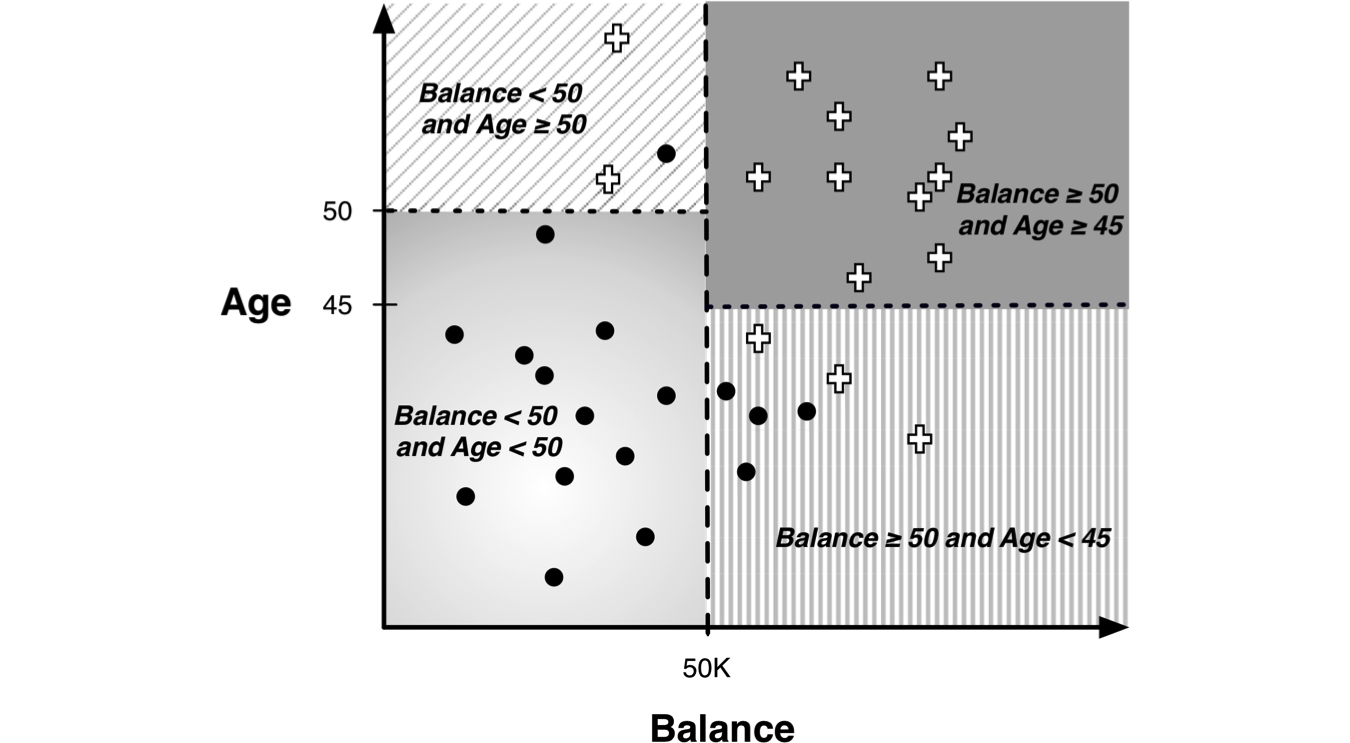
Legend: Black dots=write off; plus-sign=non-write-off
Trees as Sets of Rules
Another way to think of classification trees: a sets of rules
IF (Balance < 50k) AND (Age < 50) THEN Class=Write-off
IF (Balance < 50k) AND (Age ≥ 50) THEN Class=No Write-off
IF (Balance ≥ 50k) AND (Age < 45) THEN Class=Write-off
IF (Balance ≥ 50k) AND (Age < 45) THEN Class=No Write-off